The Curve Sets Your Attachment, Not Your Limit

The standard method for sizing a cyber program from a loss curve has two halves. Set the retention where the balance sheet can absorb the loss, and set the limit at the one-in-hundred-year figure. The first half is sound. The second is a convention borrowed from property catastrophe practice, and the curve does not derive it.

‍

The distinction matters because organizations treat both numbers as outputs of the same model, then defend a limit the model never produced. Being precise about which decision the curve settles and which it only informs is what makes the resulting program defensible at renewal and at claim.

‍

The Curve Settles the Attachment Point

‍

Attachment is a shape question and shape is exactly what a loss distribution describes. The useful feature is the transition from losses an organization absorbs as an operating cost to losses that become financial events.

‍

On many cyber distributions that transition is abrupt rather than gradual. Modeled loss sits under a million and barely moves across the lower percentiles, then rises by close to an order of magnitude across a narrow band. Attaching below that band means insuring routine operating expense, which is expensive per dollar of risk transferred. Attaching well above it means funding the first serious event internally.

‍

Peer Retention Figures Answer a Different Question

‍

A retention set to the sector median describes what comparable organizations negotiated, which is a function of their premium appetite and their broker relationships rather than of your loss distribution. The curve gives a reason. The benchmark gives a precedent, and only one of those survives a question from a chief financial officer, which peer benchmarking is better used for elsewhere.

‍

The Limit Is a Capital Question

‍

Selecting a limit means deciding how much loss the organization will not fund itself. The answer depends on liquidity, on covenant headroom, on access to credit and on what the board will tolerate reporting, none of which appears in a loss model.

‍

The one-in-hundred convention arrived from insurance capital practice, where it functions as a regulatory solvency standard rather than as a buying rule. Applied to a cyber distribution it produces a number with no particular claim to being the right one, and the shape of cyber loss differs enough from natural catastrophe that the borrowed default deserves examination rather than acceptance.

‍

Ask What Happens at the Return Period You Chose

‍

The productive version reverses the question. Rather than asking what the one-in-hundred figure is, take a candidate limit and ask what the organization does the day a loss exceeds it. Where the answer is a credit facility and an uncomfortable quarter, the limit is defensible. Where the answer is a covenant breach or an emergency raise, it is not, whatever return period it corresponds to.

‍

Nobody Decides to Retain the Layer Above the Limit

‍

Every program has an unlimited retention above its top layer, and it is almost never stated as a decision. Choosing a limit is simultaneously choosing to carry everything above it, and that half of the choice tends to go unrecorded.

‍

Writing it down changes the conversation. A board that has approved a limit has usually not been asked to approve retaining an unbounded amount above it, and presenting both halves together occasionally produces a different answer. It also gives the risk function something to point at later, since a documented acceptance is a materially better position than an implied one, and an appetite statement that can be breached is where that acceptance belongs.

‍

Sub-Limits Are Where Programs Fail in Practice

‍

An aggregate limit can be perfectly adequate while the program still fails to respond, because the loss lands against a sub-limit sized years ago on a different basis.

‍

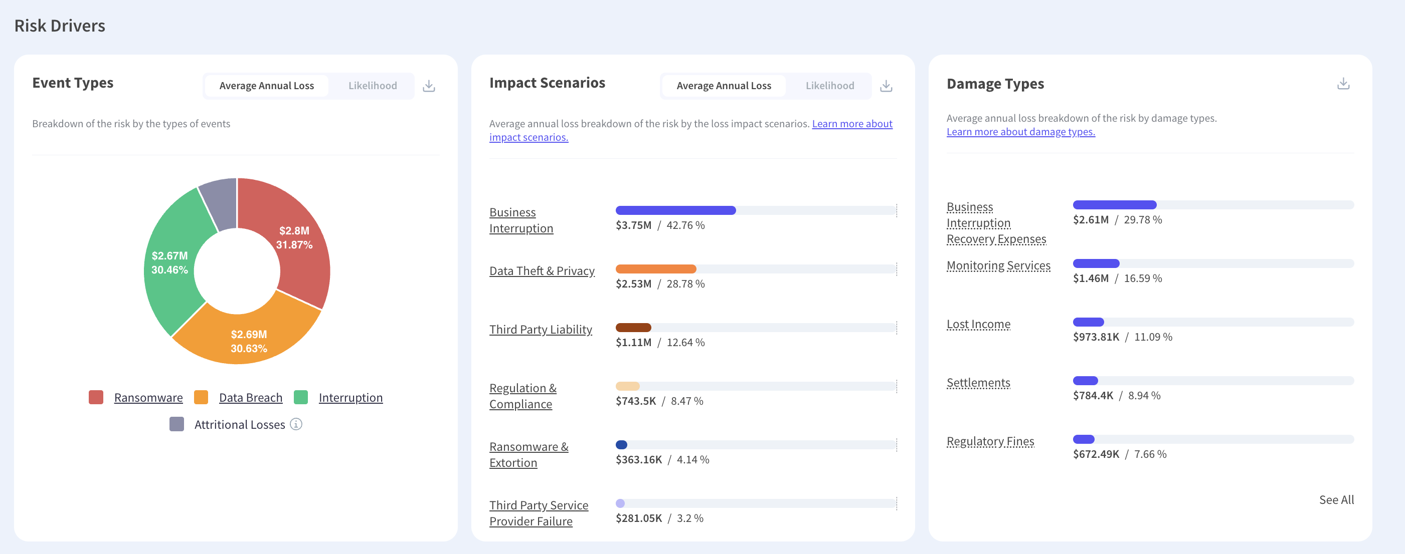
Business interruption and contingent business interruption are the usual culprits, both because they are frequently the largest component of modeled loss and because they were often sized when the organization had fewer dependencies. Modeling exposure per damage type rather than in aggregate is what exposes the mismatch, and the exercise regularly shows a program whose headline limit is generous and whose largest exposure is capped at a fraction of it.

‍

Test Each Sub-Limit Against Its Own Distribution

‍

The mechanical step is to model loss separately for each coverage line and compare the result against that line's sub-limit rather than against the aggregate. Waiting periods deserve the same treatment, since a twelve-hour waiting period against modeled outage durations concentrated below twelve hours describes coverage that will rarely respond, and reading the curve for duration rather than for magnitude is a separate exercise.

‍

Sometimes the Curve Says Do Not Buy

‍

An honest reading occasionally argues against the instrument, and an analysis incapable of reaching that conclusion is not an analysis.

‍

Where the distribution shows a substantial attritional body and a thin tail, most of the modeled loss sits in a region insurance prices efficiently against and the organization could self-fund. Premium spent transferring that region buys little, and the same money directed at reducing frequency moves the whole lower portion of the curve. Where the body is small and the tail is heavy, the reverse holds and transfer is the right instrument. The shape tells you which situation you are in, and testing whether coverage is correctly sized covers the over-purchase case specifically.

‍

What the Model Cannot Tell You

‍

Three limits belong in any presentation of this work, because a limit recommendation offered without them invites more confidence than the method supports.

‍

• Wording Decides Recovery: A modeled loss falling inside a limit still depends on the policy responding to that loss, which is a coverage question rather than a quantification one.
• Market Capacity Constrains Choice: The available limit at an acceptable price may differ from the indicated one, particularly in a tightening market.
• Correlation Sits Outside Single-Event Modeling: Two events in one policy year against a shared aggregate is a scenario a per-event view does not surface.

‍

The first is the one that costs money. An organization that sized a limit precisely and never examined whether its wording responds to the scenarios driving the figure has done half the exercise, and the exclusions that surface at claim are usually in the wording rather than in the amount.

‍

The Sequence That Works

‍

Five steps, in this order, and the order matters because each one constrains the next.

‍

Model loss by damage type rather than in aggregate. Set the attachment where the distribution transitions from routine to material. Test each sub-limit and waiting period against its own line's distribution. Take a candidate aggregate limit to the treasury function and ask what exceeding it would require. Then record the retained layer above the limit as an accepted position with a named approver. Everything before the fourth step is analysis and the fourth step is the decision, which is the part a model cannot make.

‍

Know Which Number the Curve Produced

‍

A loss distribution is unusually good at settling where a program should attach, because that is a question about shape and shape is what it describes. It is considerably weaker on the limit, which depends on liquidity, covenants and tolerance that no loss model contains, and the one-in-hundred convention is a borrowed default rather than a derived answer. Sub-limits are where programs fail in practice, the retained layer above the limit is a decision most organizations never record, and the wording determines whether any of it responds. Kovrr's cyber insurance coverage optimization models exposure per coverage line against the program as it stands, which is the view the sub-limit question requires.

‍

To see your current program plotted against modeled loss by damage type, book a demo with our risk experts.