Same Inputs, Different Answers: FAIR and Actuarial Models

Two defensible routes to a cyber loss figure exist. One decomposes a specific scenario into factors and simulates them. The other fits distributions to historical loss experience across a population and projects forward. Both are legitimate, both are in production use, and given what looks like the same inputs they produce different answers.

‍

The difference is not noise and it is not one method being wrong. Four identifiable mechanisms drive it, and knowing which one is responsible for a particular disagreement tells you which figure to use for which decision.

‍

Frequency Means Different Things

‍

The first mechanism is the one that produces the largest errors in practice, and it is usually a misuse rather than a disagreement.

‍

Factor-based analysis separates how often a threat attempts something from how often those attempts succeed, holding control strength as its own term. An actuarial approach works from observed loss events, which are already the successful subset. Feed a raw attempt frequency into a model expecting realized events and the output overstates exposure substantially, because the control term has been silently dropped.

‍

Check Which Frequency You Were Given

‍

When two analyses disagree by a large multiple, this is the first thing to test. Ask whether the frequency input describes attempts or outcomes. A great many reconciliation exercises end there, and the resolution is arithmetic rather than methodological.

‍

Distribution Choice Drives the Tail

‍

The second mechanism is the least discussed and the most consequential for anything involving a return period. Identical minimum, most likely and maximum values do not produce identical distributions once a simulation engine runs against them.

‍

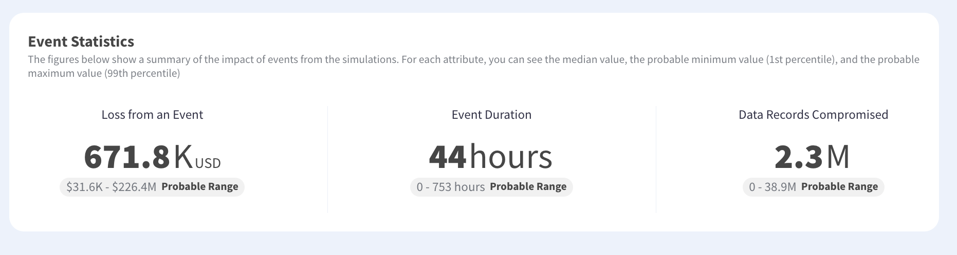
Factor-based tooling commonly uses distributions that concentrate probability around the most likely value, on the reasoning that expert estimates need constraining. Actuarial practice favors heavy-tailed families, because observed loss data across a population exhibits extreme events that a constrained distribution suppresses. Same three numbers, materially different ninety-ninth percentile.

‍

Comparing Two Outputs Compares Two Assumptions

‍

An organization holding figures from two methods and treating the difference as a matter of opinion about risk is frequently looking at a difference of opinion about distribution shape. The question is resolvable technically rather than a judgment call, and it should be settled by asking which family each engine used rather than by splitting the difference.

‍

Scope Answers Different Questions

‍

The third mechanism is definitional and produces confusion rather than error.

‍

A factor-based analysis typically evaluates one scenario at a time, stated narrowly enough that its inputs can be debated. Ransomware reaching a specific system through a specific path. An actuarial view more often produces an annual aggregate across all event types. Handed the same inputs, the first answers what this scenario costs and the second answers what a year costs, and the numbers are not comparable because they are not measuring the same object.

‍

Aggregation Is Where Scenarios Become a Year

‍

Converting a set of scenario figures into an annual position requires deciding how they combine, which is where correlation enters. Summing independent scenario losses produces an annual figure only if the scenarios genuinely are independent, and shared dependencies mean they are not, so aggregating with correlation applied gives a different answer from adding them up.

‍

Secondary Loss Is Conditional in One and Averaged in the Other

‍

The fourth mechanism concerns how consequential-but-contingent costs enter the calculation.

‍

Factor-based analysis models regulatory penalties, litigation and reputational effects as separate conditional terms that trigger only in defined circumstances. Actuarial fitting tends to absorb them into the observed severity distribution, since historical losses already include whatever secondary costs those events incurred. The first approach makes the assumption visible and debatable. The second embeds it in the data and is harder to interrogate, while requiring fewer judgments.

‍

Neither Handling Is Superior

‍

Explicit conditional terms are auditable and depend on estimates somebody supplied. Embedded secondary costs are grounded in experience and reflect the regulatory environment of the period the data came from, which for cyber may be materially different from now. Choosing between them is a choice about which weakness is more tolerable for the decision at hand.

‍

Which Figure Suits Which Decision

‍

The disagreements resolve once the question is specified, and the two approaches have different natural applications.

‍

• Control Investment Cases: Factor decomposition, because the control term is explicit and moving it shows what an improvement is worth.
• Capital and Insurance Decisions: Actuarial fitting, because those decisions turn on the tail and heavy-tailed families are calibrated to observed extremes.
• Board Reporting on Position: An annual aggregate, since directors are asking about the year rather than about one scenario.

‍

Scenario-level debate with technical teams is where factor decomposition earns most, because the structure gives a security engineer something specific to disagree with rather than a figure to accept. Scenario-based modeling and portfolio aggregation are complementary rather than competing, and a program using only one is answering a narrower set of questions than it thinks.

‍

How to Reconcile Two Numbers

‍

The wrong move is averaging them, which produces a figure neither method supports and nobody can defend. The sequence below usually locates the difference in under an hour.

‍

Establish whether the frequency inputs describe attempts or realized events. Confirm whether both outputs cover the same scope, meaning one scenario against an annual aggregate. Ask which distribution family each engine used, particularly if the disagreement is concentrated in the tail rather than the median. Check whether secondary losses are conditional terms in one and embedded in the severity data of the other. Where all four match and the figures still differ, the remaining difference is a genuine disagreement about inputs and worth having.

‍

Record the Method With the Figure

‍

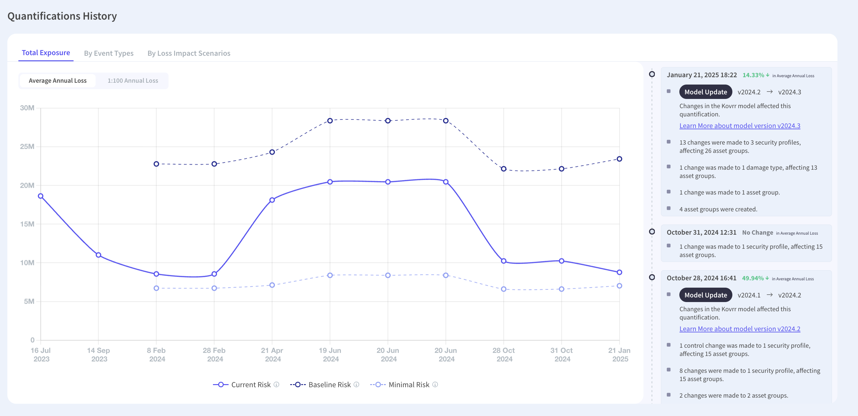
A number carried in a register without its method and version cannot be reconciled later, and movement between periods becomes uninterpretable. Whether a change reflects the environment or the model is the first question anyone asks, and model stability determines how much of the difference is signal.

‍

What Both Approaches Share

‍

The disagreements are narrower than the debate suggests. Both express risk as a distribution rather than a rating, both require frequency and severity as separate inputs, both produce a range rather than a point, and both are considerably more useful than a colored matrix.

‍

Both also depend on the same inputs being right, and neither compensates for an asset value that reflects a balance sheet from three years ago. Argument about methodology occupies more attention than it deserves relative to the quality of what goes in, and the errors that distort figures most are mostly upstream of the choice.

‍

Specify the Question, Then Pick the Method

‍

Two defensible approaches producing different answers from apparently identical inputs is not a failure of either. Frequency means attempts in one framing and realized events in the other. Distribution choice moves the tail without touching the median. Scope differs between a scenario and a year. Secondary costs are conditional in one and embedded in the other. Each mechanism is checkable, which makes reconciliation a technical exercise rather than a negotiation, and the method should follow from the decision rather than from institutional preference. Kovrr's cyber risk quantification records the model version alongside each figure so a later difference can be attributed.

‍

To see modeled exposure with the assumptions and model version behind each figure, book a demo with our cyber risk experts.